
Ancient Greek philosophers used to study mathematics, because mathematical thinking provided an ideal model of philosophical thought, free of the complications of hairier subjects in philosophy like ethics. Plato’s dialogue Meno, for example, uses a mathematical demonstration to probe the nature of knowledge. Although at times mathematics can seem like it has no connection to the real world, occasionally a deep understanding of some mathematical concepts can give clarity to our ordinary ways of thinking. One of the most beautiful examples of this comes from linear algebra.
To set the stage, we should first recall the phrase, “the map is not the territory”.
A map is not the territory it represents, but, if correct, it has a similar structure to the territory, which accounts for its usefulness.
— Alfred Korzybski
In the context of linear algebra, this concept is important for students to understand when they learn the difference between a vector and the coordinates of that vector. The reason students get confused about this in the first place is because usually the first vector spaces they are exposed to are vector spaces like  , where vectors are usually written out with notation like
  . In this special case, it is okay to identify the vector
  with a triple of real numbers, because for there is a canonical coordinate system (due to the way is constructed). In this special case, vectors really are their own coordinates (i.e., the map is the territory)!
When the Map is not the Territory
However, this breaks down once you consider other vector spaces like  , the space of polynomials of degree at most two. A polynomial of degree at most two is a function which can be written in the form
  , with
  ,
,  , and
, and  real numbers. It may be tempting to then identify
  with the triple of numbers
  , but this would be a mistake! For one, although it is possible to expand all polynomials of degree at most two in terms of
  ,
,  , and
, and  , they can also be expanded in terms of
  ,
,  , and . If we take a polynomial like
  , we could re-express it, just as validly, as
  . Indeed, a little basic algebra shows that:
![\[3(t-1)^2 + 10(t-1) + 8 = (3t^2 - 6t + 3) + (10t - 10) + 8 = 3t^2 + 4t + 1\]](https://moody.industries/blog/wp-content/ql-cache/quicklatex.com-1f7b3400787448c248bac6ac6911071c_l3.png "Rendered by QuickLaTeX.com")
This means the same polynomial , depending on which basis we expand it in terms of, could either be represented as  or
or  (among others). If Alice were to use the basis
  and Bob were to use the basis
  , and both were to identify with its coordinate vector, Alice and Bob would arrive a contradiction by the chain of equalites:
![\[\begin{bmatrix} 3 \\ 4 \\ 1 \end{bmatrix} = p(t) = \begin{bmatrix} 3 \\ 10 \\ 8 \end{bmatrix}\]](https://moody.industries/blog/wp-content/ql-cache/quicklatex.com-575c24d5b253346514ee895126f584d6_l3.png "Rendered by QuickLaTeX.com")
Resolving the Contradiction
To resolve this apparent contradiction, all we have to do is recognize that different people may map the same territory in different ways. Alice might describe the polynomial using the coordinates ““, and Bob might describe using the coordinates ““. Both are equally valid descriptions of , but they are descriptions in different descriptive frameworks (i.e., in different languages).
One way of formalizing this idea is to use a special notation for “description of an object with respect to a given descriptive framework”. If  is an object (like a polynomial), and
  is a descriptive framework (like Alice’s coordinate system), then we use the notation
 ![[x]_{\mathcal{A}](https://moody.industries/blog/wp-content/ql-cache/quicklatex.com-0199c81fbfd13129923940b5942e066b_l3.png "Rendered by QuickLaTeX.com") to denote the description of object in descriptive framework . In this notation, we can see how the contradiction above no longer goes through:
to denote the description of object in descriptive framework . In this notation, we can see how the contradiction above no longer goes through:
![\[\begin{bmatrix} 3 \\ 4 \\ 1 \end{bmatrix} = [p(t)]_{\mathcal{A}} \neq [p(t)]_{\mathcal{B}} = \begin{bmatrix} 3 \\ 10 \\ 8 \end{bmatrix}\]](https://moody.industries/blog/wp-content/ql-cache/quicklatex.com-d95ba521047d06bd6659a0a24549fd0c_l3.png "Rendered by QuickLaTeX.com")
We have no more reason to believe that ![[p(t)]_{\mathcal{A}}](https://moody.industries/blog/wp-content/ql-cache/quicklatex.com-48f850a1ddf4ee7400c20b2c4d6288d8_l3.png "Rendered by QuickLaTeX.com") (the description of in Alice’s descriptive framework) is the same as
(the description of in Alice’s descriptive framework) is the same as ![[p(t)]_{\mathcal{B}}](https://moody.industries/blog/wp-content/ql-cache/quicklatex.com-e68d56d342532ec3e71ee65b999e5995_l3.png "Rendered by QuickLaTeX.com") (the description of in Bob’s descriptive framework) than we have to believe that the word used to describe shoes in English is the same as the word used to describe shoes in French. Of course, it may happen by sheer coincidence that the descriptions of an object in two different languages are the same, but this is not to be expected.
(the description of in Bob’s descriptive framework) than we have to believe that the word used to describe shoes in English is the same as the word used to describe shoes in French. Of course, it may happen by sheer coincidence that the descriptions of an object in two different languages are the same, but this is not to be expected.
However, that doesn’t mean that the descriptions of objects in two different descriptive frameworks bear no relation at all. Indeed, if we consider the Alfred Korzybski quote above, if we know that has a similar structure to the territory, and  has a similar structure to the territory, then and should have similar structure to each other!
Deriving a Translation Rule
One way to capture the similarity in structure between two descriptive frameworks is to describe a translation between them. Using Alice and Bob’s descriptive frameworks for polynomials of degree at most two from earlier, it turns out we can derive a straightforward algebraic translation from to for any polynomial of degree at most two. Let’s derive this now.
First, let’s suppose that ![[p(t)]_{\mathcal{A}} = \begin{bmatrix} a \\ b \\ c \end{bmatrix}](https://moody.industries/blog/wp-content/ql-cache/quicklatex.com-4ee0caf0ecaff92baafb146abe12b1f4_l3.png "Rendered by QuickLaTeX.com") . Then we can derive:
. Then we can derive:
![\[p(t) = at^2 + bt + c = a\big((t-1)^2 + 2(t-1) + 1\big) + b\big((t-1) + 1\big) + c = a(t-1)^2 + (2a + b)(t-1) + (a + b + c)\]](https://moody.industries/blog/wp-content/ql-cache/quicklatex.com-2778cb52229b0d1cfe81b6f24e34072e_l3.png "Rendered by QuickLaTeX.com")
But this means
![\[[p(t)]_{\mathcal{B}} = \begin{bmatrix} a \\ 2a + b \\ a + b + c \end{bmatrix} = \begin{bmatrix} 1 & 0 & 0 \\ 2 & 1 & 0 \\ 1 & 1 & 1 \end{bmatrix}\begin{bmatrix} a \\ b \\ c \end{bmatrix}\]](https://moody.industries/blog/wp-content/ql-cache/quicklatex.com-c19c56fbd072348839155cc18a202659_l3.png "Rendered by QuickLaTeX.com")
was arbitrary, we thus derive the following translation rule for all polynomials of degree at most two:
![\[[p(t)]_{\mathcal{B}} = \begin{bmatrix} 1 & 0 & 0 \\ 2 & 1 & 0 \\ 1 & 1 & 1 \end{bmatrix}[p(t)]_{\mathcal{A}}\]](https://moody.industries/blog/wp-content/ql-cache/quicklatex.com-63c67ed749da84012283dd75bcbcc099_l3.png "Rendered by QuickLaTeX.com")
What we notice in this case is that there is a linear relationship between and . In the context of linear algebra, the translation rule between and is known as a change of coordinates, and it is described by an invertible matrix.
An Exercise to Test Your Understanding
Before reading on, try to answer the following question using your understanding of linear algebra and the Alfred Korzybski quote above:
Why is the relationship between and linear?
If you are stuck, here’s a hint: Alice and Bob’s coordinate systems are both linear coordinate systems. That is, ![[x+y]_{\mathcal{A}} = [x]_{\mathcal{A}} + [y]_{\mathcal{A}}](https://moody.industries/blog/wp-content/ql-cache/quicklatex.com-18504d1b8b297234d9e7c22201867ce7_l3.png "Rendered by QuickLaTeX.com") and
and ![[cx]_{\mathcal{A}} = c[x]_{\mathcal{A}}](https://moody.industries/blog/wp-content/ql-cache/quicklatex.com-dad09151bace80b87e0a9c0e9f4fb79c_l3.png "Rendered by QuickLaTeX.com") (and likewise for ).
(and likewise for ).
Figured it out? If not, here’s the answer. The functions ![[\cdot]_{\mathcal{A}}: p(t) \mapsto [p(t)]_{\mathcal{A}}](https://moody.industries/blog/wp-content/ql-cache/quicklatex.com-932b9c9303115aa5a3656a6217fc0ae8_l3.png "Rendered by QuickLaTeX.com") and
and ![[\cdot]_{\mathcal{B}}: p(t) \mapsto [p(t)]_{\mathcal{B}}](https://moody.industries/blog/wp-content/ql-cache/quicklatex.com-0dc2baa739912e33684479e3773827d0_l3.png "Rendered by QuickLaTeX.com") are invertible linear maps. Thus the map
are invertible linear maps. Thus the map ![[\cdot]_{\mathcal{B}} \circ [\cdot]_{\mathcal{A}}^{-1} : \mathbb{R}^3 \rightarrow \mathbb{R}^3](https://moody.industries/blog/wp-content/ql-cache/quicklatex.com-315a6e58e82d5cfb5f417cdec0d9cb82_l3.png "Rendered by QuickLaTeX.com") is linear (and invertible). Now tracing back definitions,
is linear (and invertible). Now tracing back definitions, ![\big([\cdot]_{\mathcal{B}} \circ [\cdot]_{\mathcal{A}}^{-1} \big) [p(t)]_{\mathcal{A}} = [\cdot]_{\mathcal{B}} \big( [\cdot]_{\mathcal{A}}^{-1} [p(t)]_{\mathcal{A}} \big) = [\cdot]_{\mathcal{B}} (p(t)) = [p(t)]_{\mathcal{B}}](https://moody.industries/blog/wp-content/ql-cache/quicklatex.com-a42ffc6a5974cec031d74f58ef96c07a_l3.png "Rendered by QuickLaTeX.com") , so
, so ![[\cdot]_{\mathcal{B}} \circ [\cdot]_{\mathcal{A}}^{-1}](https://moody.industries/blog/wp-content/ql-cache/quicklatex.com-af360a19e17a6080f97be207533bb317_l3.png "Rendered by QuickLaTeX.com") is indeed the translation from descriptions/coordinates to descriptions/coordinates. In plain English: the relationship between and is linear because the relationships between and and between and are both linear.
is indeed the translation from descriptions/coordinates to descriptions/coordinates. In plain English: the relationship between and is linear because the relationships between and and between and are both linear.
Picturing What’s Going On
The following diagram explains what’s going on when we translate between and coordinates, and vice versa:
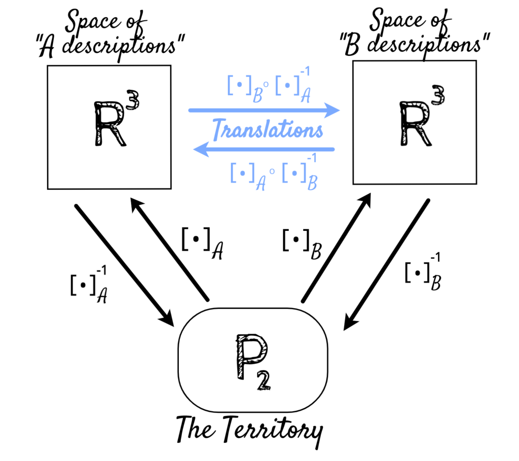
This diagram applies far more general than you might expect. If we replace with an arbitrary domain (corresponding to a territory), and the two copies of with arbitrary spaces of descriptions, then the blue formulas for translation between and descriptions are still valid, so long as ![[\cdot]_{\mathcal{A}}](https://moody.industries/blog/wp-content/ql-cache/quicklatex.com-0104ee24f168e1802196a26eba60706b_l3.png "Rendered by QuickLaTeX.com") and
and ![[\cdot]_{\mathcal{B}}](https://moody.industries/blog/wp-content/ql-cache/quicklatex.com-784a843bc0f299e067820e722aad7e20_l3.png "Rendered by QuickLaTeX.com") are bijective functions. Since and are maps from objects of the domain to descriptions, this is just another way of saying that every object in the domain has a unique -description (resp. -description), and every -description (resp. description) corresponds to a unique object in the domain. Although this is not true for natural languages (because sometimes descriptions fit more than one object, and some objects have many different descriptions), it is often true for artificial languages / descriptive frameworks.
are bijective functions. Since and are maps from objects of the domain to descriptions, this is just another way of saying that every object in the domain has a unique -description (resp. -description), and every -description (resp. description) corresponds to a unique object in the domain. Although this is not true for natural languages (because sometimes descriptions fit more than one object, and some objects have many different descriptions), it is often true for artificial languages / descriptive frameworks.
What’s special in the case of linear algebra is just that these functions and are invertible linear maps, which implies all the arrows in this diagram are invertible linear maps.